You’ve built a solid product. QA signs off. Everything checks out in the lab. Then, a few months after launch, the calls start coming in. A batch of units just failed. Then another. Some devices last weeks, others seem fine for months. Customers are frustrated. The sales team is nervous. Support is overwhelmed. And engineering is left staring at dashboards, wondering what went wrong. This is the nightmare scenario—one most reliability teams know all too well, and one that tools like the Weibull Distribution are designed to help predict.The worst part? There’s no obvious smoking gun. The failures seem random. But deep down, you can feel it: this isn’t random at all.
You’re likely examining a situation where the failure rate is changing over time, but your current metrics can’t capture it. That’s where the Weibull distribution becomes a critical tool, not just for analyzing past failures, but also for predicting future ones before they occur.
Let’s get into how it works, why it matters, and how to start using it—even if you don’t have a mountain of data.
Why MTBF and “Pass/Fail” Aren’t Telling the Full Story
Most teams rely on traditional quality checks and average failure rates, such as Mean Time Between Failures (MTBF). And those metrics are fine, as long as your failure behavior is stable and random.
But what if it’s not?
Imagine this:
- Half your units die early, within the first 300 hours.
- The rest run fine for over 2,000 hours.
- Your MTBF still shows a respectable average.
However, that average masks the true story. MTBF can’t show whether failures are front-loaded, spread out, or clustered at the end of life. And “pass/fail” QA tests? They just tell you if a unit survived a specific test, not how it behaves over time.
That’s why smart reliability engineers go a step further. They turn to time-to-failure analysis. Specifically, the Weibull distribution—because it adapts to different types of failure behavior and gives you insight into how things are failing.
What the Weibull Distribution Does (and Why It’s So Useful)
The Weibull distribution is a statistical model that describes the likelihood of failure at various points in time. It’s incredibly flexible, and that’s its power.
Where other distributions assume a constant failure rate, the Weibull lets you model:
- Early-life failures (think design flaws or manufacturing issues)
- Random failures (external shock, stress, etc.)
- Wear-out failures (fatigue, corrosion, aging materials)
It’s based on two parameters:
- Shape parameter (β): This tells you how the failure rate changes over time.
- Scale parameter (η): This gives you a time reference, like when most failures start to occur.
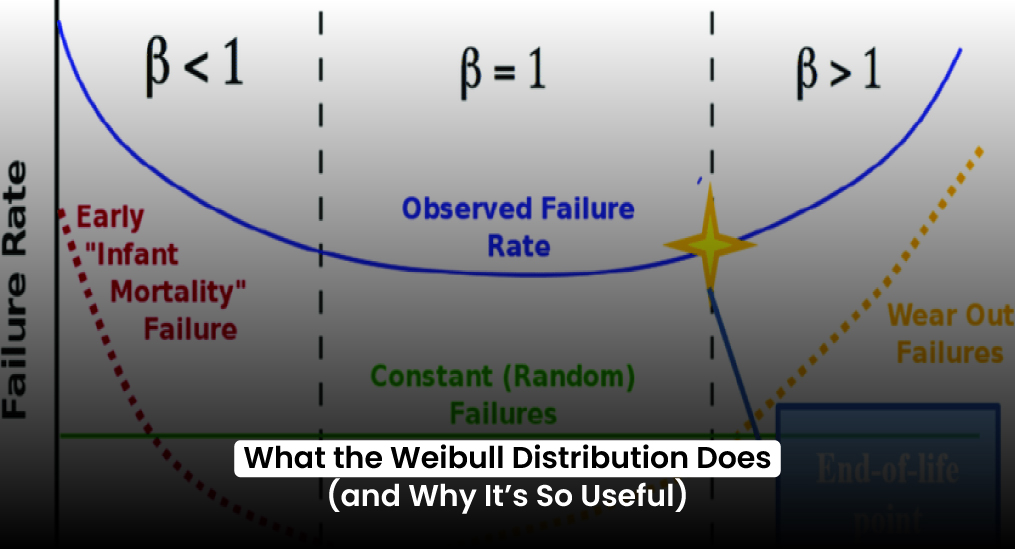
Here’s how the shape parameter (β) helps you interpret the failure behavior:
- If β < 1, failures decrease over time (infant mortality).
- If β = 1, failures occur at a constant rate (random failures).
- If β > 1, failures increase with time (aging or wear-out).
That’s the insight most teams are missing. When you know how your failure rate is evolving, you can:
- Pinpoint where the risk is highest
- Make smarter design or material decisions
- Forecast warranty claims
- Preempt support problems
- Avoid future redesigns
The Weibull distribution doesn’t just help you explain what happened. It gives you tools to act before things go sideways.
What Weibull Can Tell You That QA Can’t
Let’s say you run HALT testing, thermal cycling, shock testing, and pass everything. No units fail in the lab. Everyone breathes a sigh of relief.
But field use is messy. Customers aren’t handling your product the same way your lab techs did. And environmental factors? You can’t control humidity in a warehouse or the temperature swings in a delivery truck.
QA is a gatekeeper. It protects against obvious failures. But it’s not predictive. It can’t tell you if a part will survive past 2,000 hours or die at 300.
Understanding your product’s failure rate, not just whether it passes QA, is crucial when customers rely on consistent performance in real-world conditions.
That’s the gap the Weibull distribution fills.
It transforms raw failure timing into a timeline of risk. And that timeline helps you model what’s likely to happen next, not just what’s already happened.
Real-World Example: From Confusion to Control
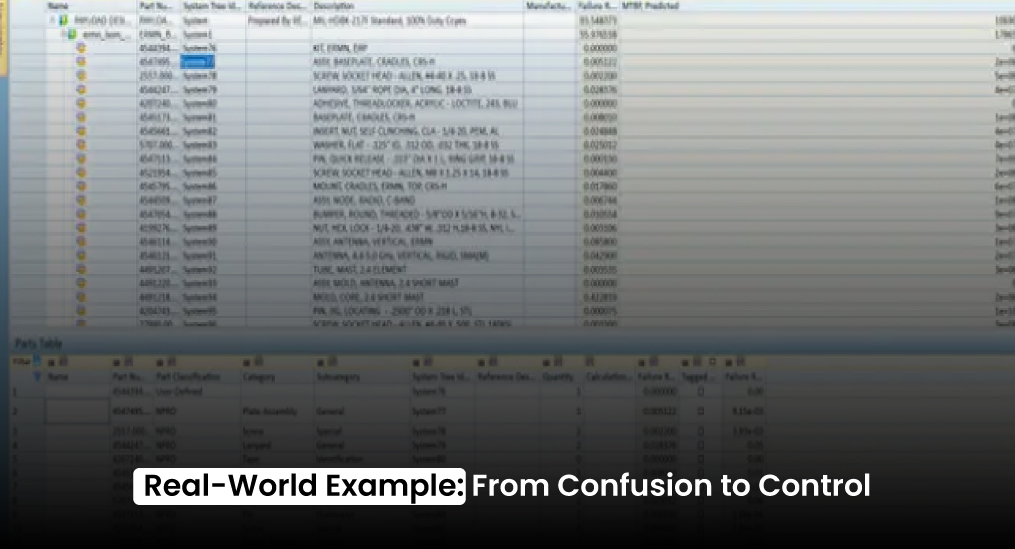
Let’s take a case from a real mid-size electronics firm.
They had just launched a new wearable sensor. Within the first 90 days, customer complaints began to trickle in. Units stopped working after about 5–7 weeks of normal use. QA logs looked clean. The assembly process was unchanged. Vendor parts were verified.
But returns kept climbing.
They collected 48 failed units and pulled their time-to-failure data. It ranged from 400 hours to about 1,200 hours. They ran a Weibull analysis and discovered a shape parameter (β) of 2.3.
That’s a major red flag.
It meant failures weren’t random—they were increasing over time. Something in the product was wearing out. When they dug deeper, they found the adhesive used to secure a sensor board was degrading in high-humidity environments, leading to stress fractures in the PCB.
Armed with this data, the team didn’t just redesign the adhesive application—they also revised their warranty forecast and re-ran accelerated life tests with the new fix.
The Weibull distribution didn’t directly fix the product. But it made the problem visible in a way no spreadsheet or MTBF average could.
How to Get Started with Weibull (Even if You Don’t Have Perfect Data)
You don’t need a lab full of test benches or hundreds of failure events to use Weibull effectively.
Here’s a simple process to get started:
Step 1: Collect Time-to-Failure Data
If you have return logs, warranty claims, or lab failures, grab the timestamp when the unit first failed.
Step 2: Include Censored Data
Censored data means units that haven’t failed yet. If a unit is still running at 1,500 hours, that’s still valuable. These observations shape the curve.
Step 3: Use Weibull Software or Tools
You can use tools like:
- Minitab or ReliaSoft (industry tools)
- Excel with Add-ins
- Python packages like scipy.stats.weibull_min or lifelines
These tools fit the curve for you and return the shape and scale parameters.
Step 4: Read the Shape
Once you have your β, you’ll know whether you’re dealing with early defects, random failures, or wear-out.
Step 5: Forecast the Future
Now comes the magic: simulate future failures. You can estimate how many units will likely fail in the next 100, 500, or 1,000 hours—and adjust your operations accordingly.
The Weibull distribution gives you a living model of risk, not just a backward-looking average.
Common Mistakes That Skew the Model
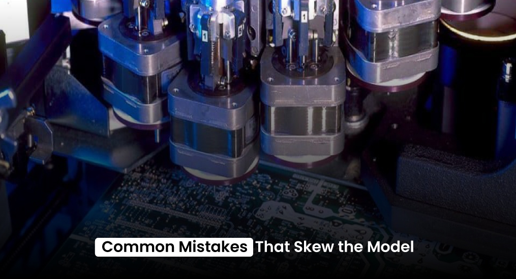
- Ignoring units that haven’t failed yet
These provide crucial boundary conditions for modeling time-to-failure. Always include them. - Assuming a constant failure rate
Most real-world failures don’t follow this pattern. Use the shape parameter to check your assumptions. - Misreading MTBF
Two very different failure patterns can produce the same MTBF. If you’re relying on MTBF alone, you’re flying half-blind. - Overfitting the model
Unless you’ve got tons of data, stick with the 2-parameter Weibull. It keeps things interpretable and grounded.
Even when using advanced methods like RBD MTBF (Reliability Block Diagram Mean Time Between Failures), you’re still limited if you can’t model time-based risk shifts the way Weibull does.
Weibull Isn’t Just for Hardware
While it’s most common in physical product testing, the Weibull distribution also applies to:
- Battery life modeling
- Software uptime behavior
- Component fatigue in mechanical systems
- Semiconductor reliability
- Medical device life cycles
In fields such as aerospace, medical devices, and industrial equipment, the Weibull distribution is often the go-to method for forecasting reliability and optimizing maintenance strategies.
Anywhere you care about how long something will last before breaking, Weibull has a role to play.
Field failures are expensive. They hurt your reputation, strain your team, and cause long-term damage to customer trust.
But they rarely come out of nowhere. Most of the time, the data is whispering the truth—you just need the right model to hear it.
The Weibull distribution helps you see what’s coming. Not in a vague, theoretical way. In a real, practical, business-relevant way.
You can predict failure patterns. You can model time-to-failure curves. You can warn your operations team before the spike hits. You can push back on overconfidence in QA and design reviews with evidence-based insight.
So don’t just report failures after they happen.
Predict them. Understand them. Plan for them.
Start using the Weibull distribution—and get ahead of the curve.